Comphy

Tutorial: Basic usage of Comphy

Welcome to the tutorial "Basic Usage".
This tutorial consists of three parts that will teach you how to:

create your own 1-dimensional MOS structure starting from the flat band diagram.
add interface and oxide charge traps to your device.
perform a simple BTI simulation.

Before we start, there are three important ground rules to keep in mind about the Comphy framework:

Comphy uses electronvolts as energy unit. All other quantities are given in Si units, (even doping concentrations are given in m⁻³).
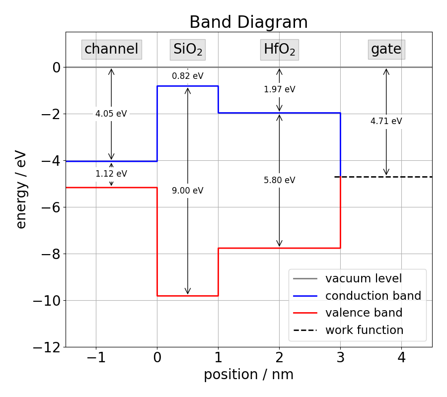
Comphy version >= 3.0 uses the vacuum level as reference level for work functions and electron affinities (see Fig. 1)
The origin of the spatial coordinate system coincides with the surface of the semiconductor and the positive x-axis points towards the gate (see Fig. 1).

comphy-band_diagram — Band structure of the tutorial device. The gate stack consists of a silicon channel, a silicon dioxide layer, a hafnium dioxide layer and a metal gate.

Prerequisites

For this tutorial we assume that you have previously activated a virtual Python environment with Comphy ready to use. If you need help setting up a suitable Python environment with Comphy, read the Installation Guide.

To start this tutorial, open a simple Python script. If you get stuck at any point in this tutorial, you can always compare your script with the Python script that accompanies the tutorial.

First import the relevant classes that we will be using in this tutorial. It is important to import the class MOS_1D first (otherwise you'll get 'cannot import ...' errors):

# import external modules
import numpy as np
import matplotlib.pyplot as plt
import scipy.signal as signal

# import Comphy modules
from src.CoreV3.MOS_1D import MOS_1D
from src.CoreV3.Physics import BandGapModel_Tdep1
from src.CoreV3.Physics import CarrierModel_Electrons_1
from src.CoreV3.Physics import CarrierModel_Holes_1
from src.CoreV3.Channel import Channel
from src.CoreV3.InsulatingLayer import InsulatingLayer
from src.CoreV3.Metal import Metal
from src.CoreV3.TrapBand import TrapBand_2S_NMP, GeneratedInterfaceTraps
from src.CoreV3.GridSampler import GaussianGridSampler, InterfaceGridSampler

# import plotting scripts
from src.Utils.Plotter import plot_band_diagram
from src.Utils.Plotter import plot_surface_potential
from src.Utils.Plotter import plot_potential_profile
from src.Utils.Plotter import plot_electric_field

# increase default font of matplotlib
plt.rcParams['font.size'] = 18