Release Consistency
The Comphy development team places a great focus on the consistency of the different releases.
However, there may be intended differences between versions, e.g. bug fixes affecting simulation results. The purpose of this chapter is to highlight desired differences between the versions and to demonstrate the overall consistency of the different versions.
Therefore, the main differences after each major update are discussed in the following section.
Version 1.0 vs 3.0The basic equations behind Comphy are:
The Poisson equation, which defines the electrostatic potential \( \phi \) in the device based on the current charge distribution \( \rho \).
The NMP rate equations describing the change of the charge distribution \( \rho \) based on the current electrostatic potential \( \phi \).
Both equations are coupled with each other, since the former fixes the electrostatic potential based on the current charge distribution
and the latter describes the change in charge distribution based on the current electrostatics.
For a correct description of charge trapping, this coupled system of equations must be solved self-consistently.
For this purpose, a self-consistent operation mode (SCP mode) was implemented in Comphy V1.0.
However, this operating mode has the disadvantage that it is computationally expensive and requires several minutes to calculate a BTI signal.
Therefore, a different approach was chosen by default in the new Comphy version.
In the default operation mode of version 3.0, the Poisson equation and the NMP rate equations are solved separately in a three-step approach:
At the beginning of each time step, the current electrostatic potential \( \phi_i \) is calculated using the current charge distribution \( \rho_i \).
Then, the rates \( k_i \) entering the NMP rate equations are determined using the potential \( \phi_i \).
Finally, the system is propagated by a time interval \( dt \) according to the NMP rate equations and the new charge distribution \( \rho_{i+1} \) is calculated.
During the last step, we assume constant rates \( k(t_i <= t < t_{i+1}) \approx k_i \). As emphasized above, this is only an approximation, since any change in the charge distribution involves a change in the electrostatic potential and thus affects the rates.
However, it turns out to be a good approximation as long as the electrostatic potential does not change significantly during the update.
If the defect density is small, this is automatically guaranteed since the effect of defects on the electrostatics is proportional to the defect density.
In the case of higher defect densities, the above condition can also be guaranteed by choosing sufficiently small time steps.
Given these conditions we were able to show that the results of version 1.0 and version 3.0 match within the limits of numerical accuracy.
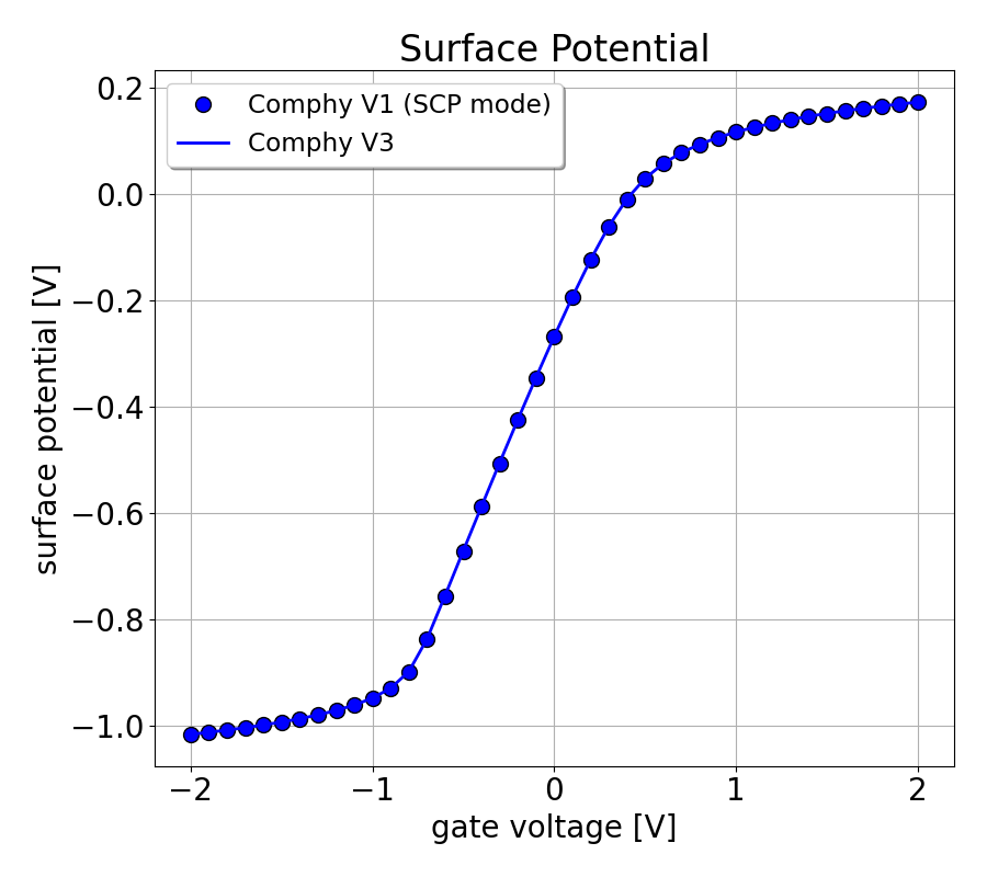
For example Fig. 1 displays the surface potential calculated with Comphy V1.0 and V3.0 for a conventional MOSFET with a 5 nm SiO2 oxide layer.
Both simulations were performed with the same initial conditions and demonstrate that the Poisson equation is solved consistently in both versions.
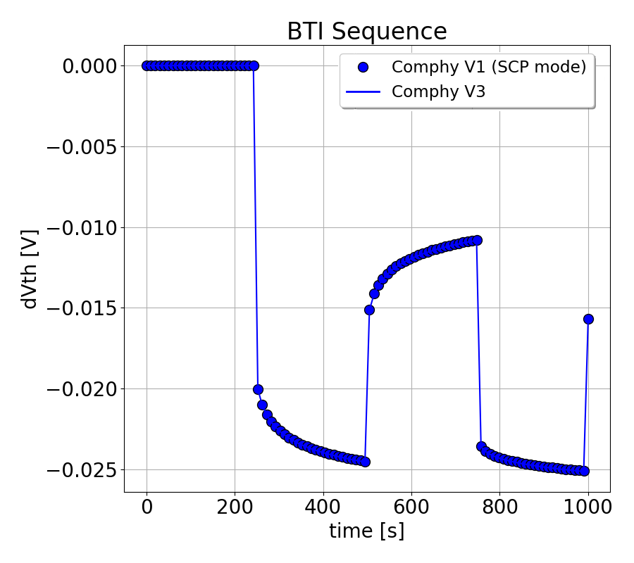
Furthermore, Fig. 2 displays the corresponding BTI sequences obtained by these simulations.
Both BTI sequences match and demonstrate that the NMP rate equations are solved consistently in both versions.
The plot shows the surface potential calculated with Comphy V1.0 and V3.0 for a conventional MOSFET with a 5 nm SiO2 oxide layer.
Both simulations were performed with the same oxide charge distribution and lead to the same surface potentials.
The plot shows the BTI sequences calculated with Comphy V1.0 and V3.0 for a conventional MOSFET with a 5 nm SiO2 oxide layer.
Both simulations were performed with the same initial conditions and lead to the same BTI sequences.