Comphy

Effective Single Defect Decomposition (ESiD)

A new approach for defect parameter extraction

One of the main motivations behind a framework like Comphy is to provide a physical degradation model based on a few measurements at accelerated stress conditions, which can then be used to estimate the device lifetime. However, in order to obtain such a model, one is usually confronted with a number of difficulties, which are briefly outlined below.

In the effective 2-state NMP model a single defect is described by the four parameters: \begin{equation} \boldsymbol{p}=\left(x_\mathrm{T}, E_\mathrm{T}, E_\mathrm{R}, R \right) \end{equation} where \( E_\mathrm{T}\) denotes the energy level of the defect, \( x_\mathrm{T}\) the the position, \(E_\mathrm{R}\) the relaxation energy and \(R\) the curvature ratio. However, most degradation experiments are carried out on large-area devices, so that only the effect of an entire defect ensemble can be observed, not the effect of individual defects. Assuming non-interacting defects, the effective threshold voltage shift \(\Delta V_\mathrm{th} \) caused by a defect ensemble can be expressed as a linear superposition of individual defect contributions \(\delta V_\mathrm{th} \): \begin{equation} \Delta V_\mathrm{th}(t,V_\mathrm{G},T)=\int N(\boldsymbol{p})\cdot \delta V_\mathrm{th}(t,V_\mathrm{G},T;\boldsymbol{p}) \mathrm{d}\boldsymbol{p} \end{equation} with an a priori unknown defect parameter distribution \( N(\boldsymbol{p}) \). Consequently, in order to obtain a well-calibrated model for the degradation of the device, one is faced with the task of inferring the a priori unknown distribution \( N(\boldsymbol{p}) \) of defect parameters from experimental measurements of \(\Delta V_\mathrm{th}\) at accelerated stress conditions. This problem statement can be recast into a non-negative linear least square (NNLS) problem: \begin{equation} N(\boldsymbol{p})=\underset{\hat{N}\geq 0}{\mathrm{arg\,min}} \left|\Delta V_\mathrm{th}-\int_\Omega \hat{N}(\boldsymbol{p})\delta V_\mathrm{th} \mathrm{d}\boldsymbol{p}\,\right|^2\, \end{equation} The naive attempt to solve the optimization problem stated by Eq. 3 would lead to solutions that are very sensitive to noise in the measurement data. To overcome this issue, previous studies often assumed that the defect parameters are distributed according to a Gaussian distribution. This assumption significantly reduces the complexity of the problem since then only the mean and sigma values of the defect parameters need to be optimized to fit the experimental data. However, enforcing an analytic form of \( N(\boldsymbol{p}) \) can lead to unphysical artifacts. In order to circumvent this issue, Comphy offers a novel approach for parameter extraction named Effective Single Defect Decomposition (ESiD), which will be described below.

In order to obtain a physically meaningful solution without enforcing an analytic form for \( N(\boldsymbol{p}) \), the optimization problem stated by Eq. 3 has to be regularized. The implementation in Comphy uses the Tikhonov approach, which introduces a regularization term that depends on the total defect density \( N_\mathrm{tot} \). With the Tikhonov approach, the term that needs to be minimized is given by: \begin{equation} N(\boldsymbol{p}) = \underset{\hat{N}\geq 0}{\mathrm{arg\,min}} \left( \left|\Delta V_\mathrm{th}-\int_\Omega \hat{N}(\boldsymbol{p})\delta V_\mathrm{th} \mathrm{d}\boldsymbol{p}\,\right|^2+\gamma^2 N_\mathrm{tot}^2 \right) \end{equation} with \( \gamma \) being an adjustable regularization parameter. The effects of \( \gamma \) on the optimization problem are twofold. One one hand, it favors solutions which require only a low defect density to match the experimental data and on the other hand, it also favours smooth solutions. In practice, a good value for \( \gamma \) can be found by plotting the total defect density \( N_\mathrm{tot} \) versus the error of the performed optimization for different \( \gamma \) values. As can be seen in Fig. 1, for too small values, the approximation error is very low at the expense of a very high defect concentration. In contrast, if \( \gamma \) is too large, there is a steep increase in approximation error when further increasing \( \gamma \). The optimal value for \( \gamma \) lies at the “corner” of the L-shaped curve, providing a good compromise between accurate representation of the experimental data with a reasonably small defect concentration.

comphy-band_diagram_traps — Impact of the regularization term 𝛾 on the obtained solutions. The optimal value for \( \gamma \) is obtained at the “corner” of the L-shaped curve, before a further increase of \( \gamma \) leads to a steep increase in the error norm of the solution.

This section was a brief summary of the publication D. Waldhoer et al. "Comphy v3.0 -- A Compact-Physics Framework for Modeling Charge Trapping Related Reliability Phenomena in MOS Devices". An in-depth description of the employed models can be found in the related publication D. Waldhoer et al. "Toward Automated Defect Extraction From Bias Temperature Instability Measurements". In order to gain a more detailed understanding of the ESiD algorthm we encourage you to read both papers.

Using the ESiD algorithm in a simulation

In this tutorial you will learn how to use the ESiD algorithm to extract defect parameters from measurement data. More specifically, you will learn how to efficiently import device parameters and measurement data, in order to correctly initialize the ESiD optimizer.

Step 1: Importing the relevant modules

Before you can use the ESiD algorithm in your own Python script, you need to import the relevant modules. To start this tutorial open an empty Python script and import the following modules:

# ESiD related modules
from Comphy.Optimizer.ESiD import ESiD
from Comphy.CoreV3.TrapBand import TrapBand_2S_NMP_ESiD

# helper modules
from Comphy.__main__ import _partofmain
from Comphy.CoreV3.ComphyBridge import device as V3Device

Step 2: Prepare measuremnt data in correct format

In order to infer the distribution of the defect parameters from the experimental data, we first have to ensure that the measurement data has the right format. Each measurement data set must be saved as a so-called time-stress file with the following tabular format:

#n t  Vg  dVth T
#u s  V  V K
0.000000000001000  -0.5  nan 425
0.000000001001000  -2.99  nan 425
0.000000010965210  -2.99  nan 425
0.000000120214896  -2.99  nan 425
0.000001318051382  -2.99  nan 425
0.000014451381909  -2.99  nan 425
0.000158447973159  -2.99  nan 425
0.001737256809792  -2.99  nan 425
0.019047648125279  -2.99  nan 425
0.208842410190570  -2.99  nan 425
2.289792000000999  -2.99  nan 425
2.291232001000997  -0.54  -0.003961323371012737 425
2.293856001000998  -0.54  -0.0033636287968579204 425
2.300704001000998  -0.54  -0.0031793755039067895 425
2.321120001000999  -0.54  -0.00256470368748718 425
2.370656001000999  -0.54  -0.001904752848599256 425
2.511072001000999  -0.54  -0.001568746921409958 425
2.906208001000998  -0.54  -0.0014124223875647823 425
3.930368001000998  -0.54  -0.0012746819560973677 425
6.834112001000999  -0.54  -0.00120204805313473 425
14.457536001000999  -0.54  -0.0014834494304144519 425

Regarding the time-stress files, please note:

The first line must start with #n and contain the names of the columns using the same names as shown above. The second line must start with #u and contain the units. No unit conversion is performed at the moment, but might be added at a later point.
If no \( \Delta V_\mathrm{th} \) measurement was carried out at a certain point in time, the corresponding entry in the time-stress file must be replaced by "nan". The framework automatically excludes the corresponding point from the fitting process.
The ESiD algorithm allows for the simultaneous fitting of multiple datasets. For this purpose, simply save the different data sets as separate time-stress files.

Step 2: Import measurement data and build the corresponding device

Next, we need to import the measurement data and build the corresponding device in the framework. To perform both tasks at the same time, we can use an input file that contains the required device parameters and references the available time-stress files. The advantage of this approach is that the Python script is not cluttered with device parameters, which contributes significantly to its readability. In addition, this approach allows quick switching between different simulation settings simply by selecting a different input file.

The following example shows the typical format of an input file. Each parameter begins with two dashes, followed by the parameter name and the parameter value separated by a space. The first part of the input file lists the necessary device parameters while the second part references the time-stress files containing the measurement data.

# device parameters
--Tinit 300
--Na_chan 1e+10
--Nd_chan 5.5e+17
--Eg0_chan 1.206
--Eg1_chan -2.73e-4
--Eg2_chan 0.0
--Egd_chan 636.0

 . . . . . .

# references to measurement data
--tsFile[0] 'table_pMOS_VgS-2.99_T125.0.crv'
--tsFile[1] 'table_pMOS_VgS-3.888_T125.0.crv'

Once we have created an appropriate input file, we can import the device parameters and the measurement data using the method _partofmain:

# select input file
inputFile = "inputFile.txt"

# import device parameters and measurement data
params, setups = _partofmain(['--paramFile', inputFile])

After this step the dictionary params contains the device parameters that were in the input file and the list setups contains the different time-stress files that were referenced in the input file. Finally, we can use the ComphyBridge module to create the device using the imported parameters:

# create MOS_1D device from parameters
my_device = V3Device(**params).device

Step 3: Initialise ESiD optimizer

The ESiD algorithm in Comphy is only used for the energetic parameters \( E_\mathrm{T} \) and \( E_\mathrm{R} \), since these parameters are most relevant for identifying possible defect candidates, while assuming that the spatial defect distribution is uniform. To use the ESiD optimizer we need to define the desired ESiD trap bands first. To initilaize the corresponding class TrapBand_2S_NMP_ESiD we need to specify the boundaries and the grid spacing for the parameters \( x_\mathrm{T} \), \( E_\mathrm{T} \), and \( E_\mathrm{R} \). In addition we need to specify the constant parameters \( R \) and \( N_\mathrm{T} \) and the trap type:

my_trapband_1 = TrapBand_2S_NMP_ESiD(

x_start=0.01E-9,	# lower bound for defect position in m
x_end=4.99E-9,	# upper bound for defect position in m
dx=2.0E-10,	# grid spacing for defect position in m
Et_min=-7,	# lower bound for defect energy level in eV
Et_max=-4,	# upper bound for defect energy level in eV
dEt=0.4,	# grid spacing for defect energy levels in eV
Er_min=0.2,	# lower bound for relaxation energy in eV
Er_max=5,	# upper bound for relaxation energy in eV
dEr=0.4,	# grid spacing for relaxation energy in eV
R=1.0,	# curvature ratio
Nt=2.0E21,	# defect density in m⁻³
trap_type='donor',	# type of traps
device=my_device,	# the device object

)

Now we can initialize the ESiD class with the device and the trap bands we created in the previous steps. In addition, we need to define a set of \( \gamma \) values the optimization should be performed for. Moreover, we have to specify the output directory in which the output data of the optimization should be stored.

E = ESiD(

device=my_device,	# the device object
gamma_min=-9,	# minimum gamma value
gamma_max=-5,	# maximum gamma value
gamma_N=15,	# number of gamma steps
outputDir='./Results',	# directory where the output will be saved
setups=setups,	# list containing time-stress data
params=params,	# dictionary containing device parameters
trapband_list=[my_trapband_1],	# list of ESiD trap bands

)

Step 4: Run optimization

Finally, we can execute the ESiD optimization with the following command:

# run optimizer
E.optimize()

This command iterates over the specified set of \( \gamma \) values and runs the ESiD algorithm for each individual \( \gamma \) value. During each iteration, a brief summary similar to the one below is printed. The summary shows the gamma value of the current iteration, the maximum error of the fit, the r.m.s error of the fit, the defect density, and the combined norm (product of maximum error, r.m.s error and defect density):

INFO: #########################################
INFO: Iteration Number = 00
INFO: Gamma = 1.000e-09
INFO: Max. Error = 2.582e-04 V
INFO: R.M.S Error = 9.977e-05 V
INFO: Estimated Nt(0) = 2.178e+27 m⁻³
INFO: Combined Norm = 5.612e+19 V²m⁻³
INFO: output data written to path ./Results/ESiD_run_1/00
INFO: #########################################
INFO: #########################################
INFO: Iteration Number = 01
INFO: Gamma = 3.162e-09
INFO: Max. Error = 2.597e-04 V
INFO: R.M.S Error = 1.026e-04 V
INFO: Estimated Nt(0) = 5.386e+26 m⁻³
INFO: Combined Norm = 1.436e+19 V²m⁻³
INFO: output data written to path ./Results/ESiD_run_1/01
INFO: #########################################
. . . .

Step 5: Analyze output data

During each iteration, various output files are saved in a separate sub folder of the main output directory './Results/ESiD_run_id/'. At the end of the run, the output data of the iteration with the minimal combined norm will be copied to the sub folder './Results/ESiD_run_id/final', resulting in the following output structure:

The following section will describe the content of the various output files in detail:

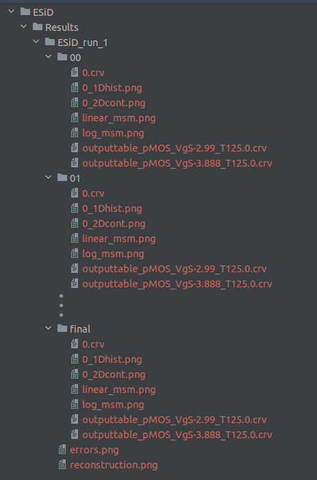
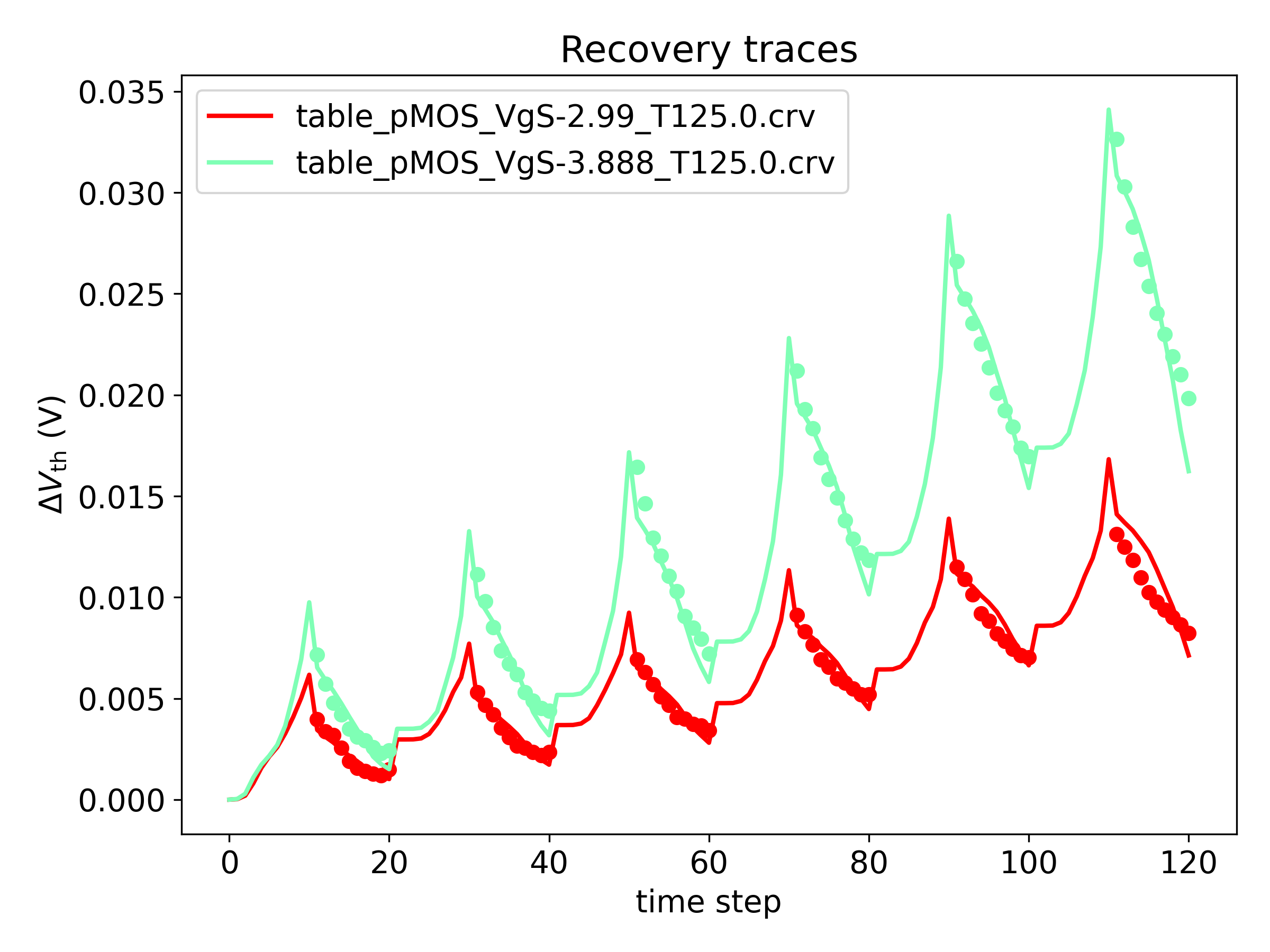
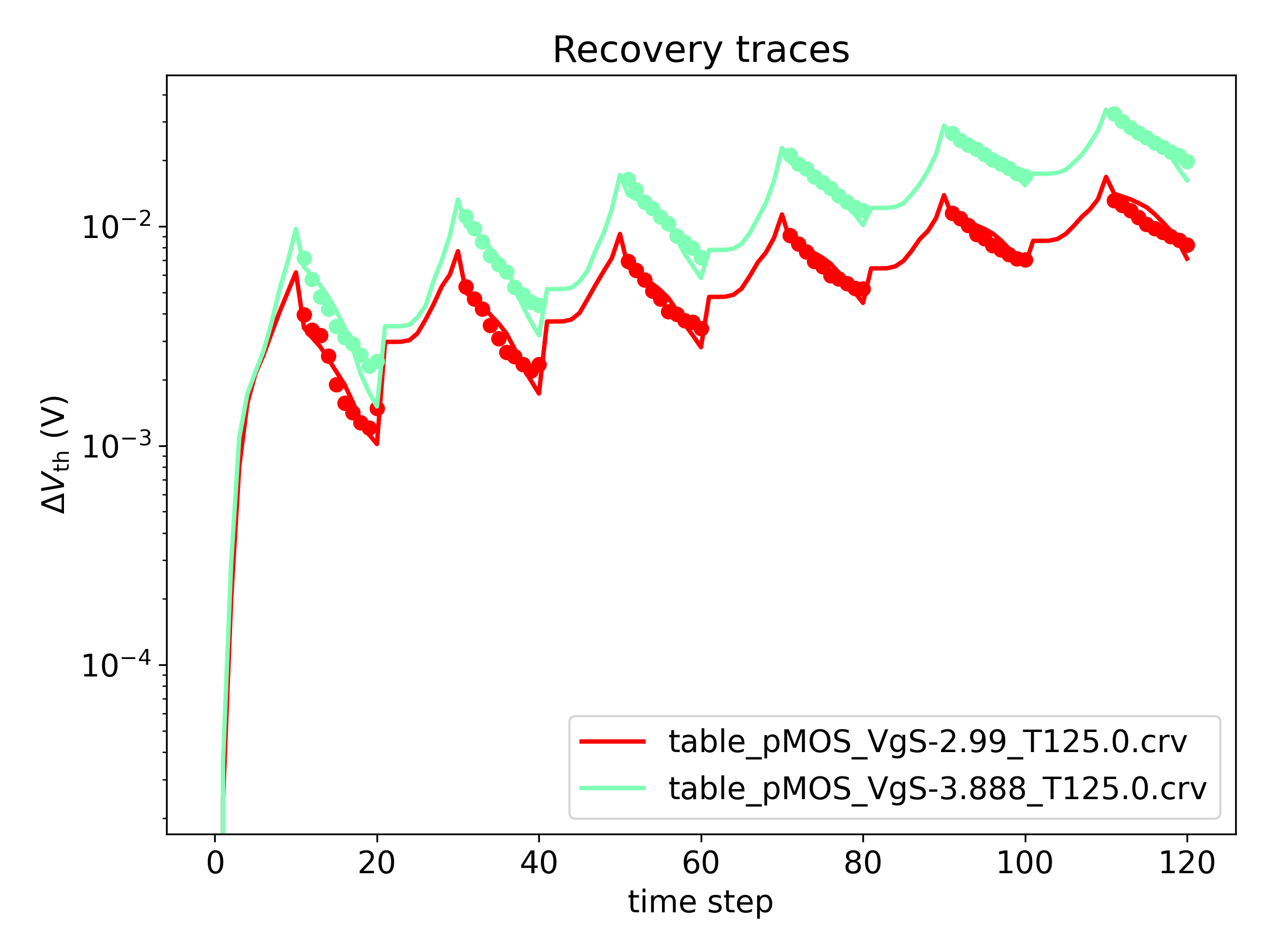
Plot of measured and fitted \( \Delta V_\mathrm{th} \)

Each output folder contains two plots that show a comparison of the measured and fitted threshold voltage shift.

The plot 'linear_msm.png' shows the mentioned comparison with a linear y-scale:

The plot 'log_msm.png' shows the above comparison on a logarithmic y-scale:

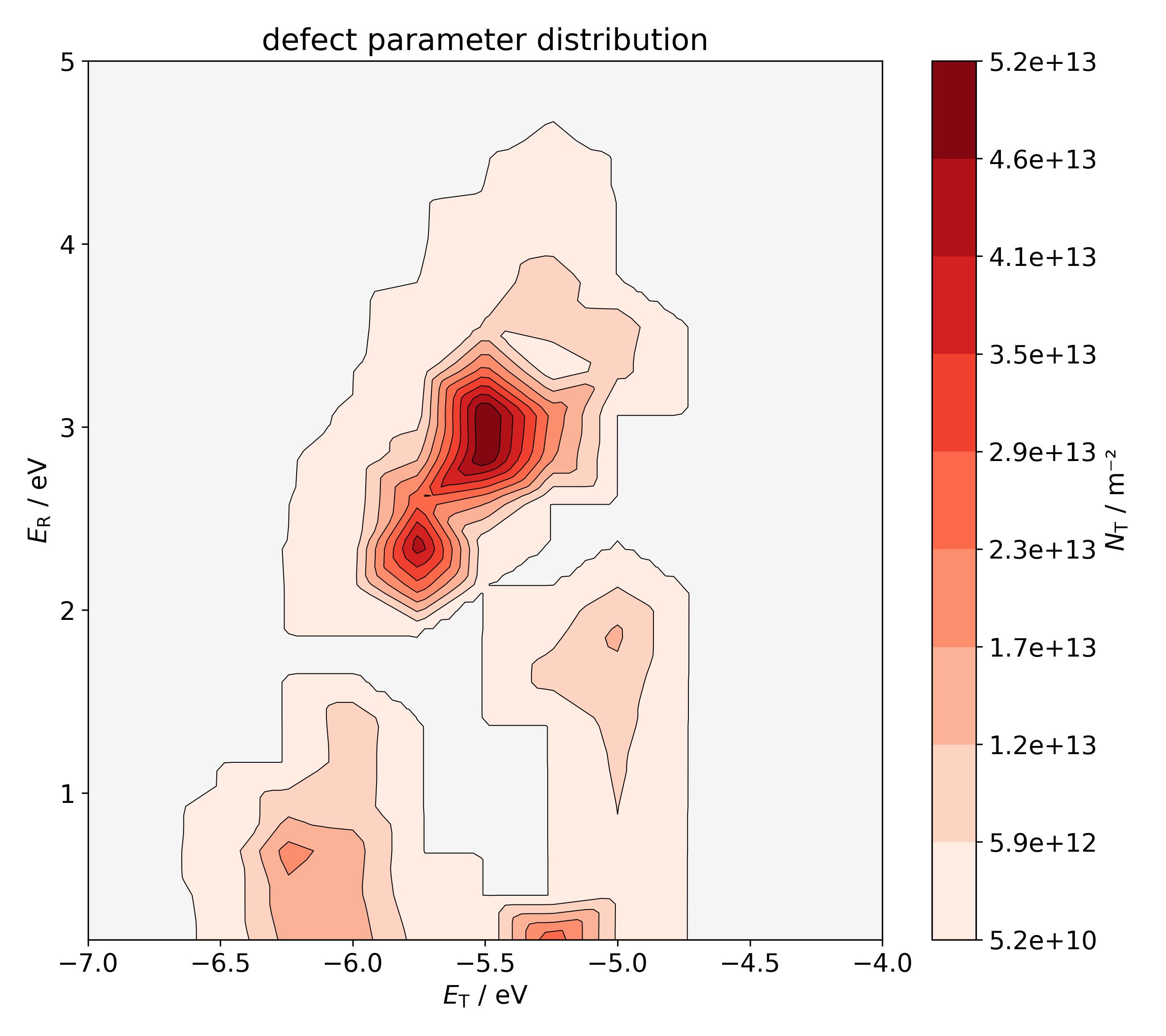
Fitted defect parameter distibutions

In addition, each output folder contains plots showing the extracted defect parameter distributions of the different trap bands. The files belonging to different trap bands are distinguished by an index, which reflects the order in which the trap bands were added to the ESiD optimizer. The following two files are created for each trap band:

The plot 'i_2Dcont.png' shows a continuous contour plot of the defect parameter distribution \( N( E_\mathrm{T}, E_\mathrm{R}) \) of the ith trap band. Since the defect densities are only known on the discrete grid used for the optimization, linear interpolation is applied to construct this continuous plot:

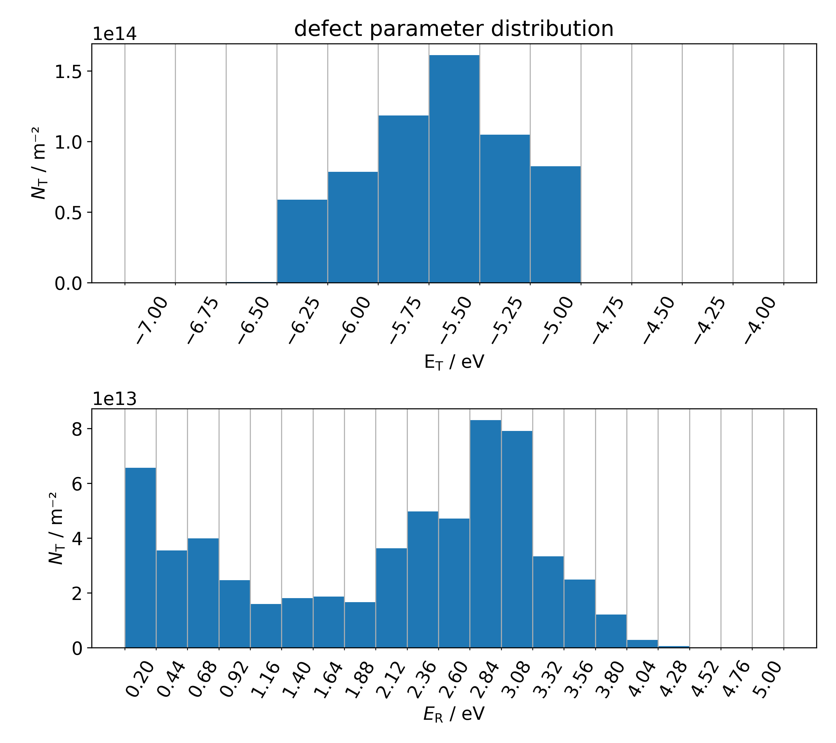
In addition, the file 'i_1Dhist.png' shows the one-dimensional projections of the defect parameter distribution \( N( E_\mathrm{T}, E_\mathrm{R}) \) of the ith trap band:

time-stress file containing the measured and fitted \( \Delta V_\mathrm{th} \)

In addition, each time-stress file used for the fit, is copied to the output folder with file name prefixed with 'outputtable_'. However, in addition to the original data, the fitted threshold voltage shift is also stored to enable further processing:

# Version: 3.0

#n	ts	Vg	dVthSim	T	dVthMeas
0.000000000	-0.500000000	0.000000000	425.000	nan
0.000000001	-2.990000000	-0.000103815	425.000	nan
0.000000011	-2.990000000	-0.000893064	425.000	nan
0.000000120	-2.990000000	-0.002742621	425.000	nan
0.000001318	-2.990000000	-0.004521839	425.000	nan
0.000014451	-2.990000000	-0.006204676	425.000	nan
0.000158448	-2.990000000	-0.008219382	425.000	nan
0.001737257	-2.990000000	-0.009891099	425.000	nan
0.019047648	-2.990000000	-0.010742648	425.000	nan
0.208842410	-2.990000000	-0.011003577	425.000	nan
2.289792000	-2.990000000	-0.012035140	425.000	nan
2.291232001	-0.540000000	-0.003731345	425.000	-0.003961323
2.293856001	-0.540000000	-0.003027215	425.000	-0.003363629
2.300704001	-0.540000000	-0.002487522	425.000	-0.003179376
2.321120001	-0.540000000	-0.002163318	425.000	-0.002564704
2.370656001	-0.540000000	-0.001966182	425.000	-0.001904753
2.511072001	-0.540000000	-0.001879344	425.000	-0.001568747
2.906208001	-0.540000000	-0.001831552	425.000	-0.001412422
3.930368001	-0.540000000	-0.001800012	425.000	-0.001274682
6.834112001	-0.540000000	-0.001752228	425.000	-0.001202048
    . . . .

error plot

Finally the main output folder './Results/ESiD_run_id/', contains a plot 'error.png' showing the evolution of the max. error, the r.m.s error, the estimated defect density and the combined norm, for debug purposes:

Plot of measured and fitted \( \Delta V_\mathrm{th} \)

Fitted defect parameter distibutions

time-stress file containing the measured and fitted \( \Delta V_\mathrm{th} \)

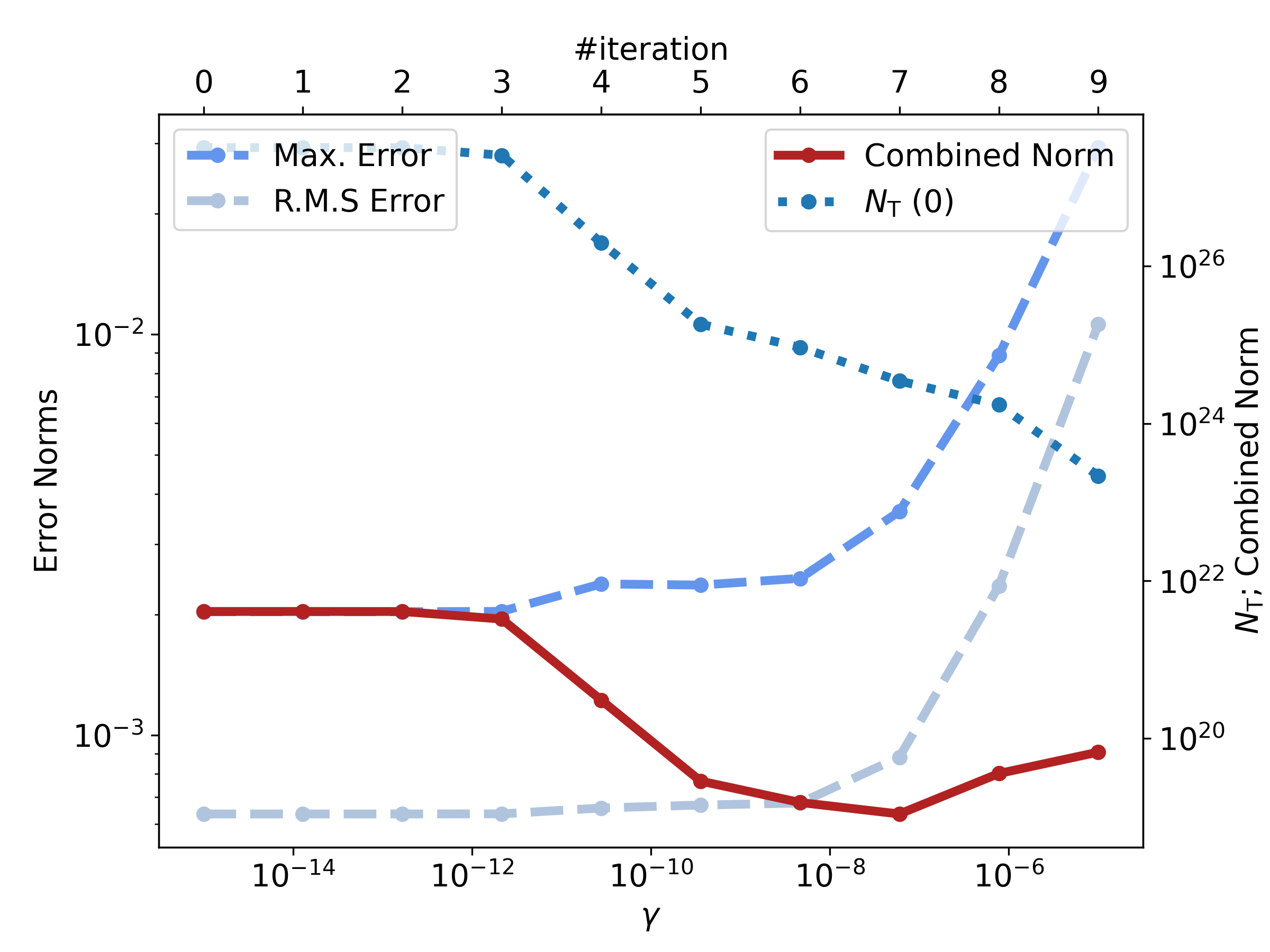
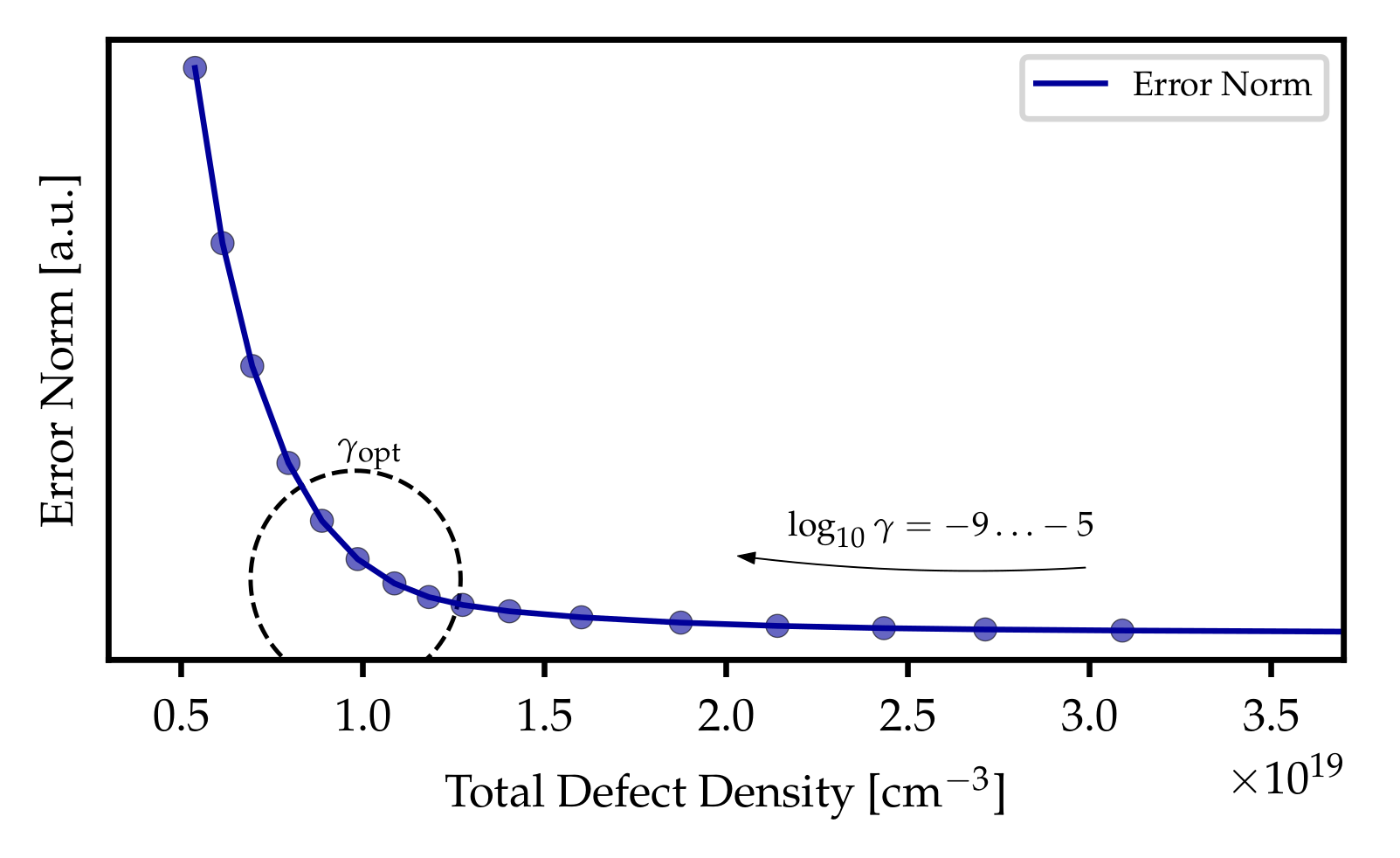
error plot